![]()

![]()


This GitHub repository contains the binary installation files (Apple OSX & Microsoft Windows) and the Matlab source code for the metabolomics standalone application QC:MXP written by Professor David Broadhurst. You can cite this package as follows:
Broadhurst, D.I. (2025). QC:MXP Repeat Injection based Quality Control, Batch Correction, Exploration & Data Cleaning (Version 3.0) Zendono. DOI: 10.5281/zenodo.11101541 Retrieved from https://github.com/broadhurstdavid/QC-MXP.
QC:MXP is FREE and you do not need to have Matlab preinstalled to use it. It is built on top of the free Matlab Runtime library, which is automatically installed.
- Introduction
- Tidy Data
- QCRSC - Quality Control Regularised Spline Correction
- QC-RSC Explorer - learn how to optimise QCRSC
- Operational Workflow
- QCRSC Configuration Options
- Batch Explorer - examine the effects of both the within-batch and between-batch correction
- Correct the whole data set
- Data Cleaning & Exploration
- Configuration File
- TUTORIAL VIDEO
- CHEAT SHEET
- How to Download & Install QCMXP
- Source Code
Introduction
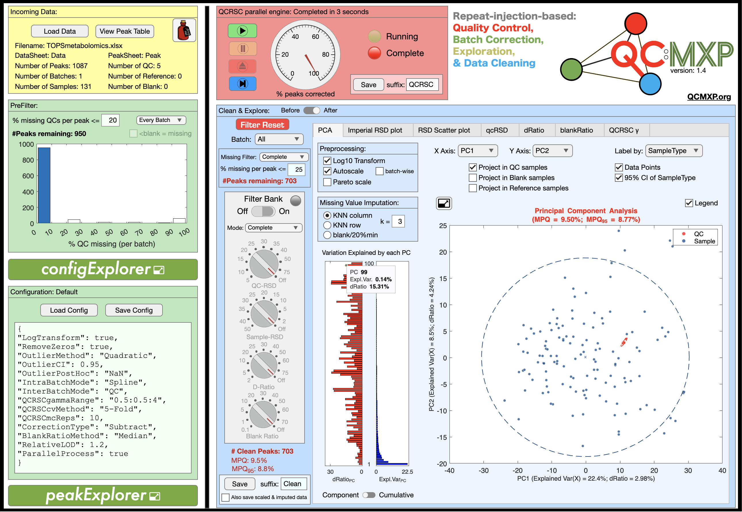
This standalone application is written specifically for the metabolomics community (but is applicable to any quantitative, or relative quantitative, multi-analyte assay that uses repeat-injection reference samples to assess repeatability). It is a long overdue companion app to the publication “Guidelines and considerations for the use of system suitability and quality control samples in mass spectrometry assays applied in untargeted clinical metabolomic studies” Metabolomics 14, 72 (2018). It can be used as an educational tool to explore the process of within-batch and between-batch correction based on repeat-injection reference samples (e.g. pooled quality control samples); however, it is designed primarily to be used as a practical tool for real world problems. It has been written as a standalone application (Mac OS, Windows 10, & Windows 11) rather than as a set of command line R or Python packages, because I wanted it to be user friendly, placing all of the cognitive load on understanding the underlying concepts, providing process transparency, and creating a highly visual interactive exploration of the data, rather than placing the majority of the cognitive load on programming skills and often frustratingly installing package dependencies. As you can see from the screenshot there are many options, which may seem daunting. However, foundational knowledge is scaffolded through interactive Explorer windows, and extensive beta testing has suggested that the learning curve is shallow. That said, it is worth noting that the process of batch correction, quality control, and data cleaning is non-trivial and requires some thought, education, and project-specific investigation.
Tidy Data
The starting point for this software is a data matrix of S samples × M features, where features are analyte concentrations, aligned features (i.e. generated by XCMS, Compound Discover etc) or similar. This matrix is linked to a table explaining the characteristics of each feature (ID code, full name, HMDB number, etc). The data can come from any platform (GC-MS, LC-MS, NMR, etc) but must be converted to my standardised QC metabolomics data sharing protocol TidyMetqc* which is an extension of my generic metabolomics data sharing protocol TidyMet* derived from the Tidy Data framework developed by Wickham 2014. This format splits the information into a tidy Data Table (feature matrix + associated sample meta data) and tidy Feature Table (feature explanations). These tables can be stored as Sheets in an Excel spreadsheet or as two .csv files. Details on these formats can be found here and multiple examples are provided in the testdata directory. Here is a brief example (NB: the feature IDs must be unique and link the two tables. In this case the first 7 metabolites acquired from an LC-MS in C18 Negative mode):
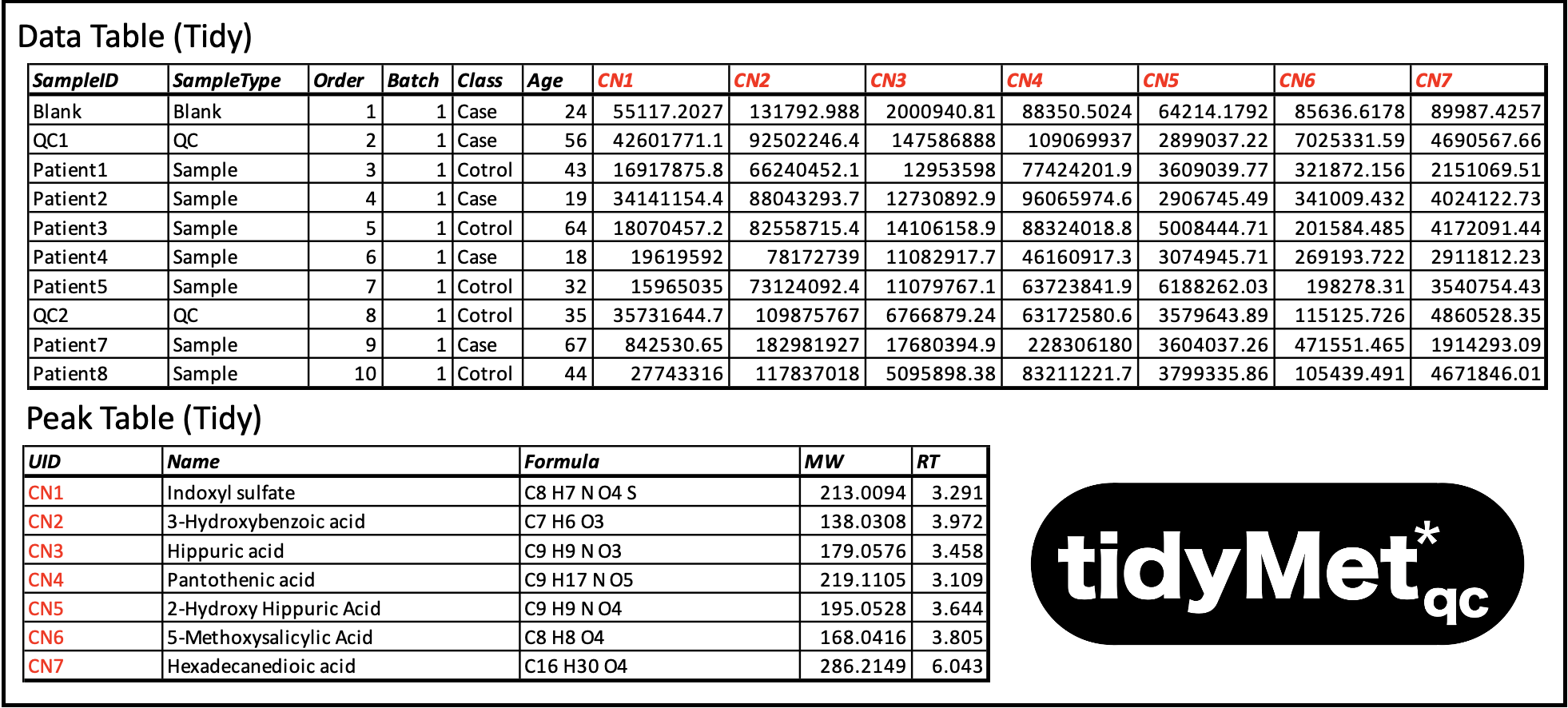 Note: The TidyMetqc* DataTable minimally requires columns: “SampleID”, “SampleType” (‘Blank’, ‘QC’, ‘Reference’, or ‘Sample’), “Order” (injection order) and “Batch” (batch number). In the example above, Columns ‘Class’ & ‘Age’ are included just to illustrate how this protocol allows a mixture of experiment data, domain metadata, and metabolite features. FeatureTable minimally requires only columns “UID” and “Name”.
QCRSC
The engine that powers the application is called QCRSC - Quality Control Regularised Spline Correction. The algorithm is based around the use of regularised (smoothing) cubic splines to model the within-batch variation in metabolite concentration for repeat-injection QC samples with respect to injection order. The (biologically identical) QC samples are assumed to accurately represent the systematic bias (sample concentration ‘drift’) and random noise (in the measurement process). The algorithm operates on each feature independently and sequentially. The basic command line version of this software (written by me) was first reported here & was an algorithmic improvement (speed, elegance, & robustness) of my first signal correction algorithm QC-RLSC Quality Control Robust Loess Signal Correction discussed in Dunn, W., Broadhurst, D., Begley, P. et al. Procedures for large-scale metabolic profiling of serum and plasma using gas chromatography and liquid chromatography coupled to mass spectrometry. Nat Protoc 6, 1060–1083 (2011). QCRSC has been used, by me, to correct many metabolomics data sets (>90) over the last 10 years, and has been adapted (often poorly) by several 3rd party groups over the years. The original QC-RLSC & QCRSC algorithms were implemented using the Matlab scripting language. Code has always been available on request, although I have generally performed data correction for people as a free service due to the bespoke nature of the process. It is only now that I have found time to release the algorithm in a form that I was happy share with the world without my direct supervision.
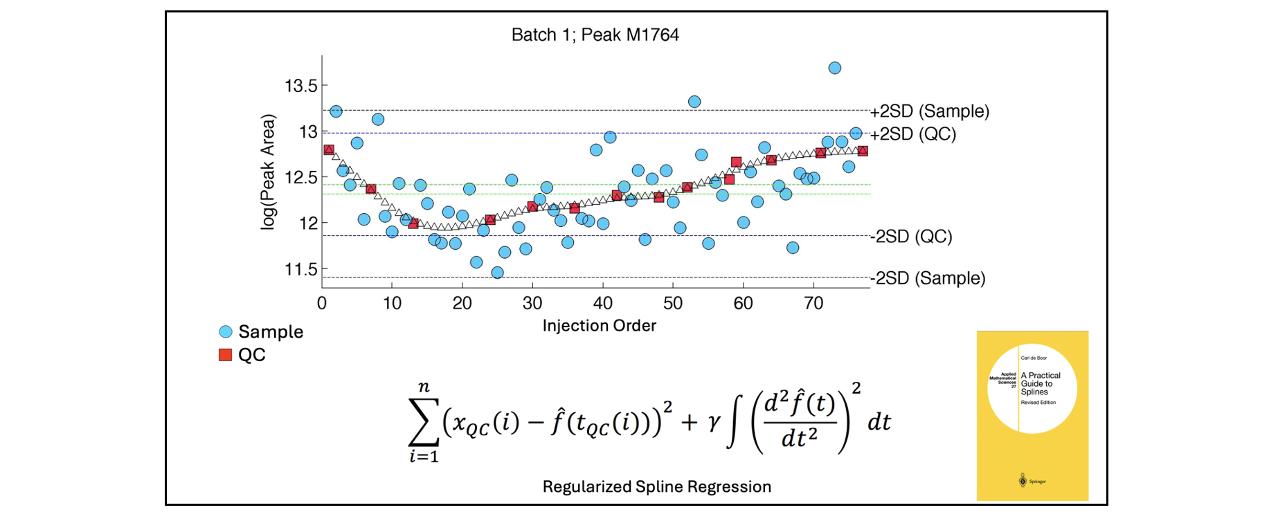
The backbone of QCRSC is a cubic spline function written by Carl de Boor (A Practical Guide to Splines. Springer-Verlag, New York: 1978). The original code was written in Fortran and called “SMOOTH”. It is available as part of PPPACK. It was then implemented by Matlab as CSAPS. It is this version of the function that is used here. For anyone interested, there is a Python modified port of CSAPS available here. The degree of linearity in the spline (regularisation) is dependent on a smoothing parameter. A very small value overfits a very nonlinear curve to the QC data points and conversely a large value removes nonlinearity completely and fits a simple linear regression. Automatic selection of the smoothing parameter is important to balance the bias-variance trade-off. This is done using cross-validation. If there is fewer than 5 QCs in a batch, or if the user does not want to use non-linear correction, a ‘Linear’ correction option has been implemented (using Robust (bisquare) linear regression). Alternatively, within-batch correction can be ignored by disabling QCRSC (also called ‘median correction’). In this case between-batch correction aligns batches based on the within-batch median QC value.
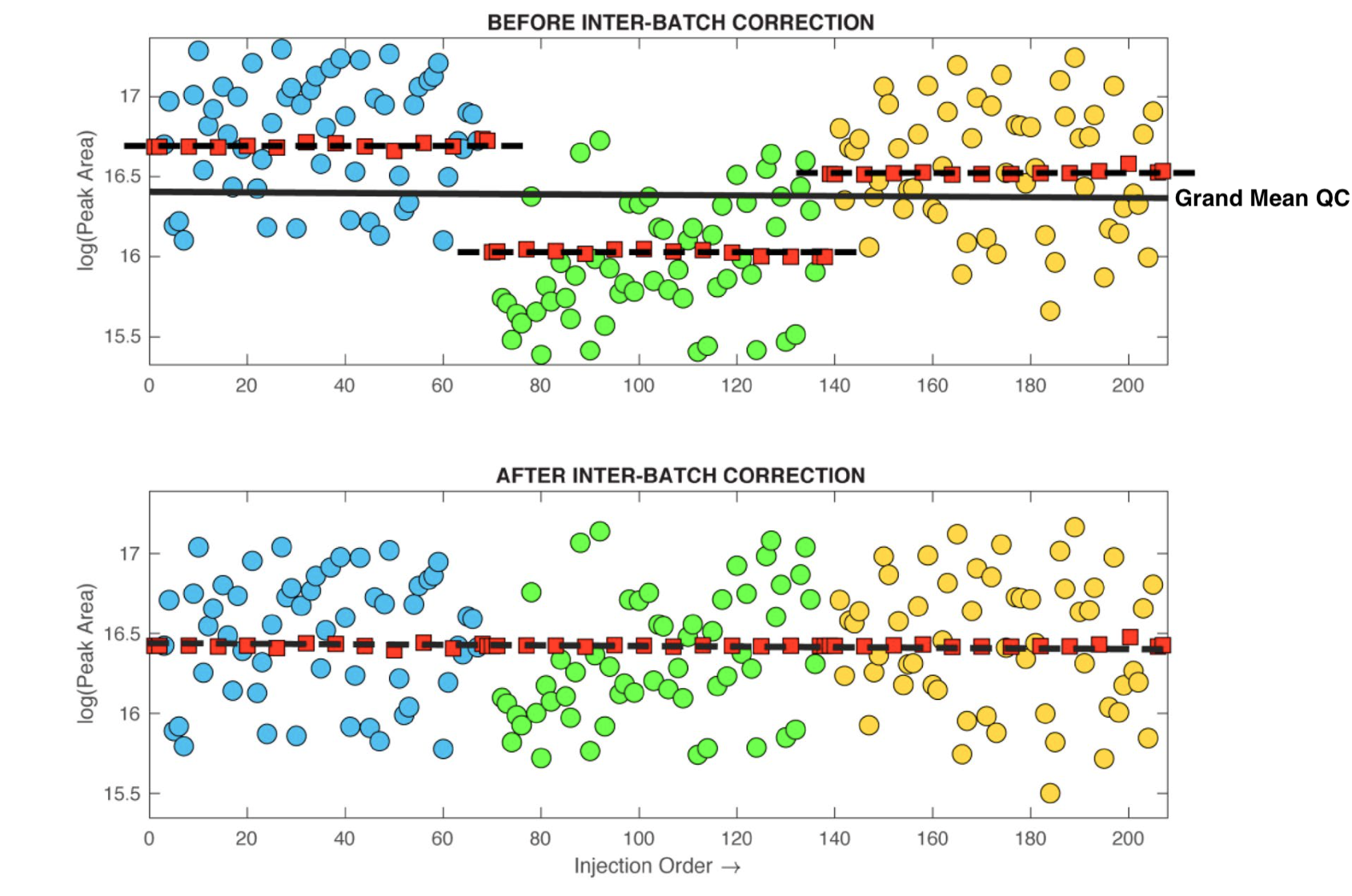
Between-batch correction is comparatively simple. Once the within-batch bias has been subtracted (or divided), batches are simply concatenated such that the median of the QC values in each batch are equalised across all batches - please refer to the figure below (adapted from the guidelines paper). NOTE: In the latest version of QC:MXP it is possible to use different sets of pooled QC samples for within-batch and between-batch correction. Each batch can have a unique set of pooled QC to perform the non-linear correction and then a “long-term” pooled QC (Reference QC) can be used align the multiple batches. The repeat-injection Reference samples must be from a single source and must be injected across all batches (preferably at least 3 injections per batch). It is worth mentioning that the performance using an independent between-batch Reference QC is (even in ideal conditions) dependent on the number of Reference QCs in each batch. The number of QCs massively influences the accuracy of the between-batch median correction. As such the use of between-batch Reference QC correction is only recommended if it impossible to use a single pooled QC across all batches.
To summarise: QCRSC operates on each feature (metabolite) independently. For each feature, it is a two-stage process of within-batch correction (linear or non-linear) followed by between-batch alignment. The within-batch spline correction requires the optimisation of a smoothing parameter for each batch (e.g. 3 batches requires 3 individual smoothing parameters for each feature).
Footnote: There are many published alternatives to QCRSC. I am not going to list them here. Many claim to be superior based on comparison of only a couple of specific data sets. I would suggest that, given sufficient QC data, it is likely that most are equally ‘fit for purpose’ within reasonable confidence intervals. More important is the lab-based design of experiment (i.e. number of samples in a batch, number of QCs in a batch, frequency of QC, inclusion of sufficient Blanks). Any nonlinear correction algorithm is going to be crippled by a low number and/or frequency of QC sample injection. So, ‘if in doubt’ use a simple batch-wise ‘linear’ correction method over any complex machine learning method. Finally, be wary of any method that celebrates the ability to automatically detect batches. IMHO batch identity is as easy to provide as the injection order, so should be used by the algorithm.
IMPORTANT: Before running QCRSC please ensure that any lead-in QCs (conditioning QCs) and lead-out QCs (ID QCs) have been removed from the data set. These samples are usually included at the start and end of every batch. Including these data will compromise the effectiveness of the QC correction algorithm. However, ideally before processing, each batch should begin and end with two pooled QC (please refer to Broadhurst et al. (2018) for details). If spline correction is performed and batches do not start and end with QCs there is a danger of some pretty wild non-linear extrapolation. In those cases you may wish to experiment with constrained spline correction (“Spline-C2”, Spline-C4” or “Spline-C6”). You have been warned!
QC-RSC Explorer
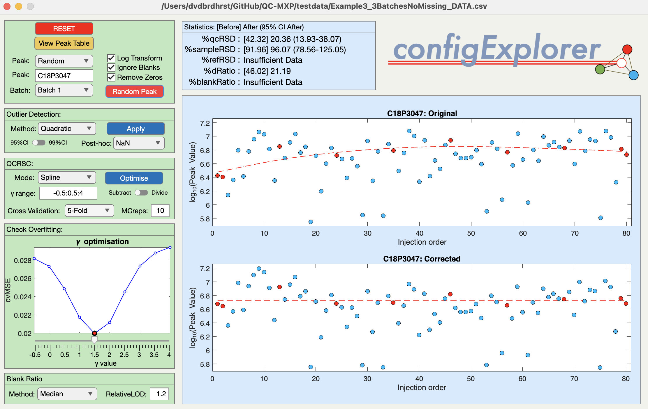
A great way to understand the underlying principles of within-batch correction is to push the button labelled QC-RSC Explorer before importing any of your own data. This launches the QC-RSC Explorer window with some artificially generated example data (see below). Pressing the red button labelled Random Feature randomly selects one of 20 metabolite features. The right-hand side of the window (gold) shows the before/after control charts for that feature (sample concentration vs injection order). The left-hand side of the window (pink) provides an interface to the QCRSC configuration options. This is a highly interactive sandbox allowing you can familiarise yourself with the basic functionality - so ‘go play!’. Hovering over buttons/boxes will trigger pop-up information windows to help explain the functions. The options will be discussed in more detail in the TUTORIAL VIDEO.
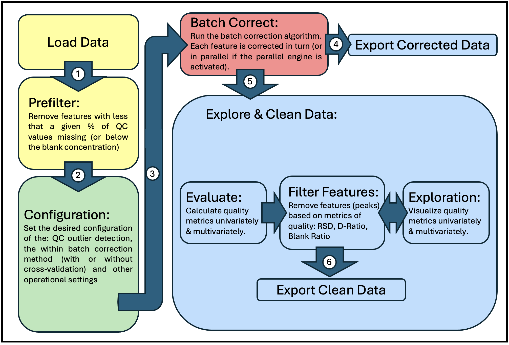
Operational Workflow
The figure below represents the general operational workflow for running QC:MXP (mapped to the corresponding location in the application window).
 Once you have imported your own TidyMet* data it is advisable, as a beginner, to again open Config Explorer. This time your own data is presented for configuration exploration (click on the batch number you want to look at). Depending on the number of QCs per batch, or the blank responses, or specific characteristics of data generated by your metabolomics platform & deconvolution software (e.g. XCMS), you may want to change the type of outlier detection, within-batch correction method (and cross-validation method), or blank ratio assessment method. The software is designed to be very flexible. Remember The configuration settings apply to all the features in the data set, across all batches, so you must review several metabolites (hit the “Random Feature” button) across multiple batches to settle on the “best” configuration settings. This is also an opportunity to observe any unwanted artefacts that repeat across multiple features (e.g. bad samples, or unexpected change in instrument sensitivity). NB The default settings have been specified based on many years of experience across many data sets from many labs. So if in doubt just keep the default.
Feature Inclusion PreFilter
The Feature Inclusion PreFilter enables the user to filter out features with poor QC representation (< % QC missing), either across all batches or for a specified number of batches (e.g. for a feature to pass there must be less than 20% missing QCs in 5 or more batches). There is an optional feature to force any QC response below a given hypothetical Limit of Detection (LOD) to be classified as missing. The LOD is defined as some multiple of the maximum data value labelled as “Blank” in a given batch. This option is best investigated using the QC-RSC Explorer app. The Feature Inclusion PreFilter can be completely disabled if so desired.
QCRSC Configuration Options
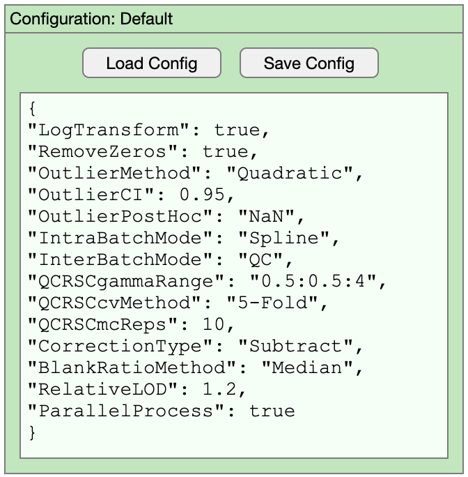
When you are happy with all the QCRSC configuration options, close the window and if you have made changes, you will be asked if you want to transfer the setting to the main application. Once back in the main window, it is advisable to save the current configuration settings before proceeding. The QCRSC configuration can also be edited from the main window should you wish to make any changes without opening the explorer. Configuration options are stored as plain text (.json file) to enable users to transparently archive the settings making them readily available for publication or repeat processing. The function and choices for each configuration option is explained in the CHEAT SHEET
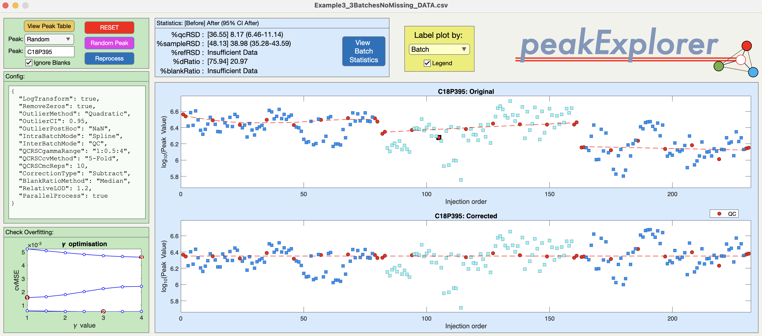
Batch Explorer
Before applying QCRSC to the complete data set it is worth opening Batch Explorer. This window is similar to QC-RSC Explorer in that you can investigate the effects of the configuration setting on individual metabolite features. However, now you can look at the effects of both the within-batch and between-batch correction.
Correct the whole data set
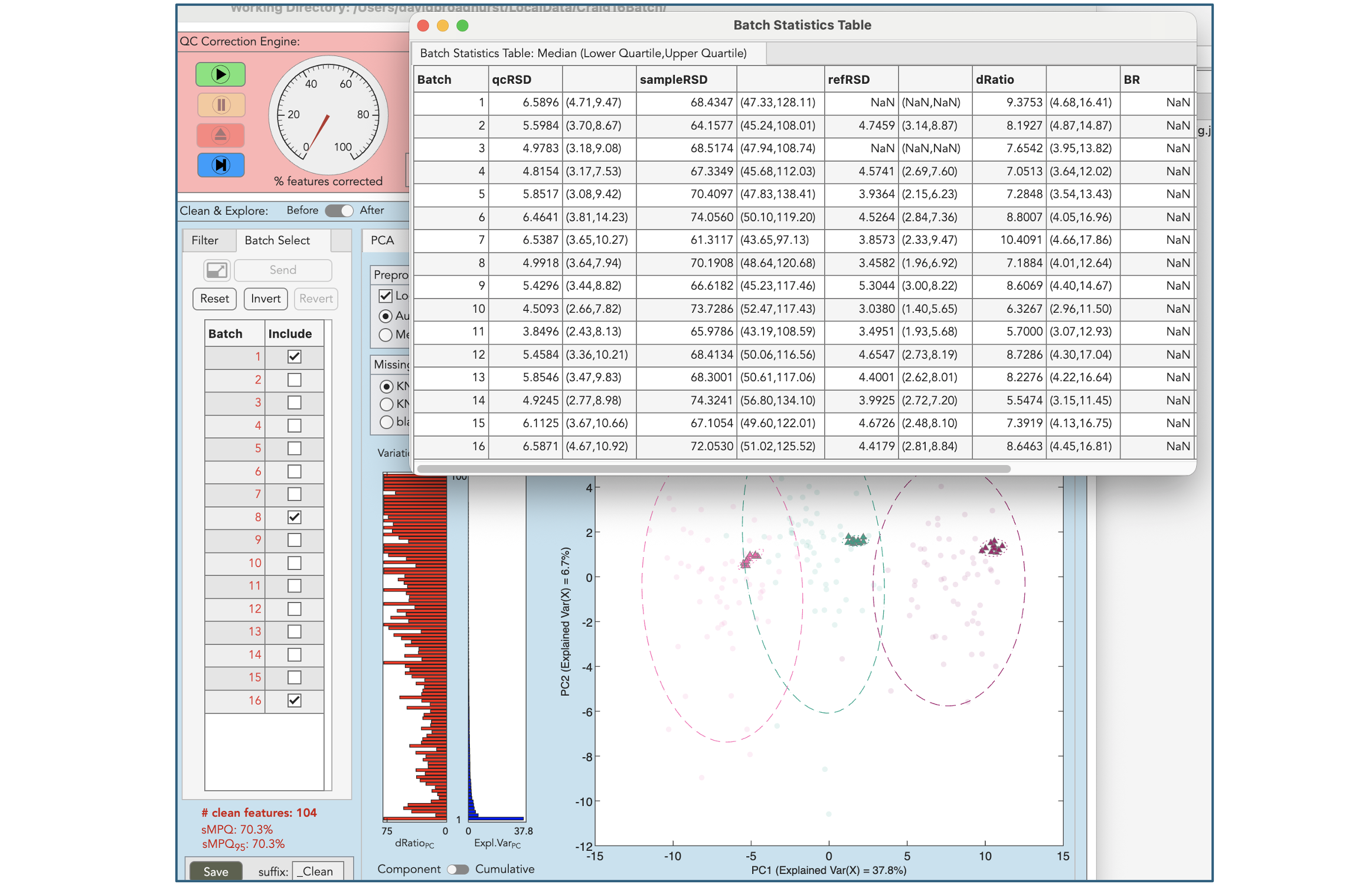
To run QCRSC on the whole data set press the green ‘play’ button on the QCRSC engine. The QCRSC algorithm will be applied sequentially to each feature in the data set. Upon completion a new corrected Data table has been created and the Feature table has been updated to include basic statistical measures (QC-RSD, D-Ratio, Blank Ratio, percent missing etc). It is advisable to save the corrected data at this point. Note an additional Statistics Table is saved which contains an exhaustive set of statistics for each individual batch and across all batches.

Batch Selection
New to version 3 is the ability to select subsets of batches to explore in isolation. Click the ‘Batch Select’ tab and select those batches you wish to include (or exclude) from analysis and then “Send” the resulting list to the visualisation windows. This feature was requested for investigating studies with a large number of batches. To help guide the inclusion/exclusion process a new pop-out ‘Batch Summary Statistics’ window has also been implemented.
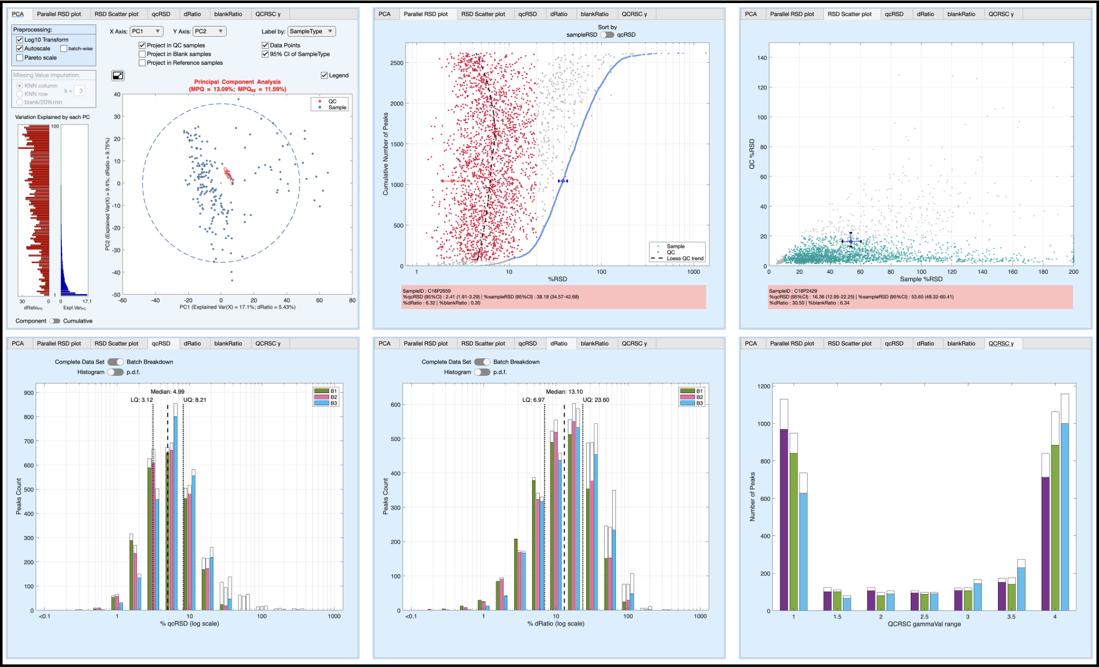
Data Cleaning & Exploration
Once the QCRSC engine has finished attention shifts to the data cleaning filters and visualisation tabs. Features (metabolites) can be filtered (removed) by ‘Number of missing values’, ‘RSD threshold’, ‘D-Ratio threshold’, and ‘Blank-Ratio threshold’. Typical settings are: Missing < 20%, QC-RSD < 20%, D-Ratio < 40%, Blank-Ratio < 20%. The effects of the QCRSC correction + filtering are shown in multiple tabs. Interpretation of these plots are discussed in the TUTORIAL VIDEO. Once you are happy with the data cleaning process, save the resulting Data table and Feature table.
Configuration File
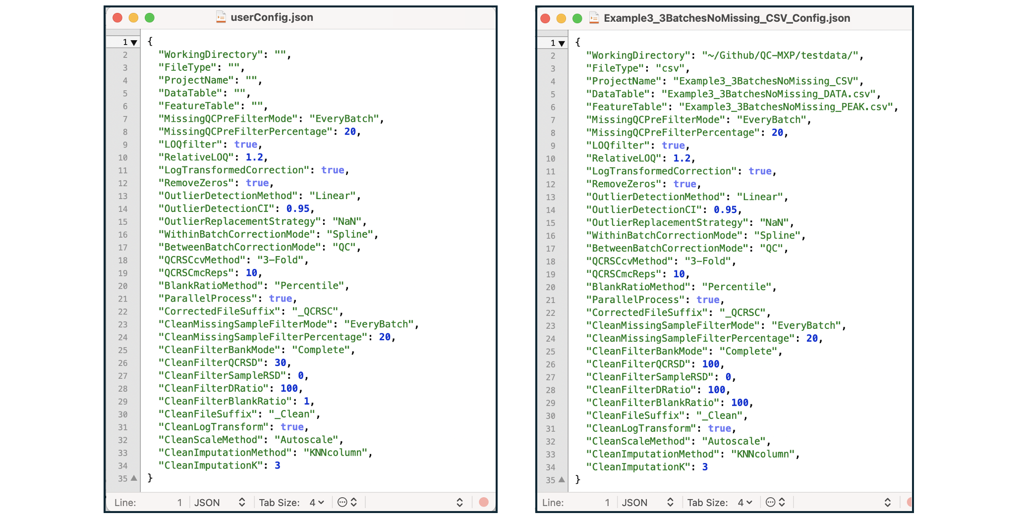
The QC:MXP app is built around a user/project configuration object. The default generic configuration is established automatically. Once user data is uploaded the configuration switches to project mode. Every completed project will have an associated configuration file containing all the settings across the whole QC:MXP workflow (filenames, project name, prefilter settings, QCRSC settings, cleaning settings). It is possible to load a whole project with data and settings from a configuration file and it is also possible to save a generic user config file to use as a starting point for subsequent projects. The project file also acts as a record of the QC:MXP workflow for reporting purposes.
TUTORIAL VIDEO
A brief tutorial for version 1.4 of QC:MXP A Data-Driven Framework for Metabolomics Quality Control was presented to the “Chemometrics & Machine Learning in Copenhagen” YouTube channel. Thanks again to Rasmus Bro for inviting me to speak. I will upload more detailed tutorials for the latest to my own YouTube site soon.
CHEAT SHEET
There is a pdf explaining the QC-MXP & QCRSC options here. This can also be accessed from within the app using the CHEATSHEET button.
How to Download & Install QCMXP
The binary installation files are found in the latest release section of the repository. Choose the one that matches your operating system (Apple Intel or Apple Silicon, Windows 10, Windows 11, or Matlab App). Download (unzip if Apple) and run. The helper app will guide you through installation. Note: For Apple users, once installed, application can be found in ‘/Applications/QCMXP/application’ (unless you customized your install). Maybe pin the app to your Dock once opened.
This application is free, but is built on top of the Matlab Runtime libraries (also free). This means installation can be slow as the runtime libraries must first be installed. It also takes while to launch (without a splash screen). This is particularly true on the first time of running. So please be patient. Do not be alarmed by any Matlab processes running in the background. This is completely normal. Any minor update to the software will not require updating the runtime libraries so will install very quickly.
Source Code
This software was developed using the Matlab App Designer. All the Matlab source code can be found in the mlapp directory. It is probably not the best documented code. The core QCRSC code is ‘QCRSC.m’ & ‘optimiseCSAPS.m’ (and of course csaps.m) & maybe ‘OutlierFilter.m’ for the outlier detection algorithms (primarily based on Matlab polyfit functions). The only other thing of note is the preprocessing & missing value imputation for the PCA plot (‘PCApreprocessing.m’). KNN imputation is either based on the Matlab function knnimpute or an incremental KNN algorithm written by me, but inspired by Ki-Yeol Kim et al.. Everything else is window dressing :-).